Introduction

This week in Election Analytics, we are talking about the ground game, or the impact that campaign operations on the ground have on election outcomes.

First, looking at the literature, there are a lot of opinions and research about different goals of the ground game, but most of them focus on persuasion, convicing a registered voter to vote for your preferred candidate, or mobilization, getting a campaign’s supporters out to vote. In their research, Professors Ryan Enos and Anthony Fowler found that presidential campaigns increased turnout substantially in highly targeted states, by around 7 or 8 percentage points on average. In comparison, Joshua Kalla and David Broockman found that campaigns have extremely low persuasive effects, amounting to an average of zero. Given this evidence, I decided to focus my analysis this week on the persuasive impact of campaigns on turnout.

Originally, my plan was to create two models, one for states that had expert predictions and one that did not, using this as an indicator for swing states. However, in their analysis, Enos and Fowler coded a “Battleground” binary variable to indicate whether intense campaigning occurred in a given state, based on Sides and Vavreck’s research. These also happened to be key swing states. I decided to mimic their method and code a similar variable, creating one model for battleground states based off of turnout, expert predictions and incumbency, and another for non-battleground states with just historical results and incumbency.

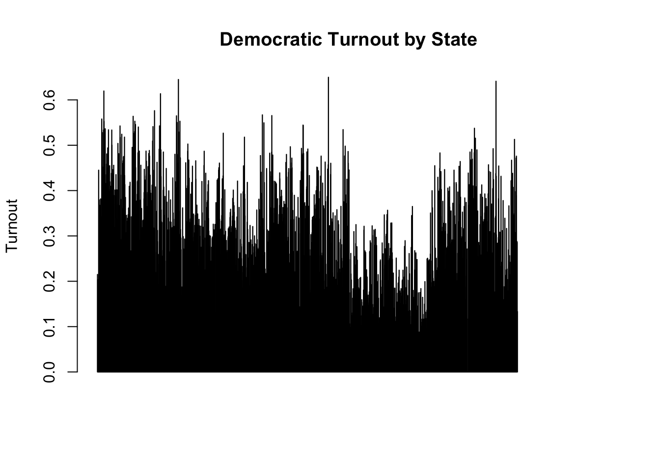
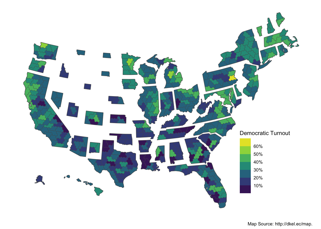
Before we dive into the models, let’s look at the distribution of turnout. First, I made a bar plot showing the turnout per state. This isn’t the most helpful bar plot but it shows us generally that Democratic turnout varies widely depending on the state. Next, I made a shaded state map that visually depicts turnout per state. This map is very cool because it sizes the districts relative to population. This map reflects that not many states have high voter turnout, and geography somewhat impacts whether a district will turn out, with the Northeast having high turnout and the South having low turnout.

Models

Moving onto my models, I followed the plan that I explained earlier, dividing the states into battleground and not battleground in order to create separate models. I was originally going to include expert predictions in the model for battleground states, except that I found there to be way too much missing data that skewed my model. I decided that it would be better to rely on turnout as this would give an accurate picture of the impact of campaigns without the conflicts of all of the secret variables taken into account in expert predictions.

I kept running into an issue where a few lines of missing data would prevent my entire model from running, so I ended up dropping the rows with missing data, which unfortunately decreased my pool of train data considerably. For next week, this is something I plan to work on to debug so I can apply a similar method again.

Conclusion

I thought that my models worked well until I reached the prediction phase and received an error about digit alignment. However, I then ran into issues with the stargazer. At this point, I am considering scrapping the district-level approach because it seems to elicit more errors than actual predictions.

Based on the data that I’ve seen this week, I believe that turnout is a useful predictor for the election as it reflects campaign efforts pretty accurately. I plan to incorporate incumbency and turnout into next week’s prediction post.