on
Blog 5: The Air War
This blog is part of a series related to Gov 1347: Election Analytics, a course at Harvard University taught by Professor Ryan D. Enos.
This week, Gov 1347 is looking at the Air War: the neverending battle between campaigns to capture potential voters’ attention via television advertisements. There are different theories about the impact of campaign ads on voting preferences but both Gerber et al. and Huber and Arceneaux, our authors for the week, have discovered through their research that ads have little to no effect on voter mobilization. Huber and Arceneaux also found that ads are strongly persuasive as to candidate choice, while Gerber et al. clarified that this persuasive impact is extremely short-lived, contributing to the increase in ads immediately before the election.
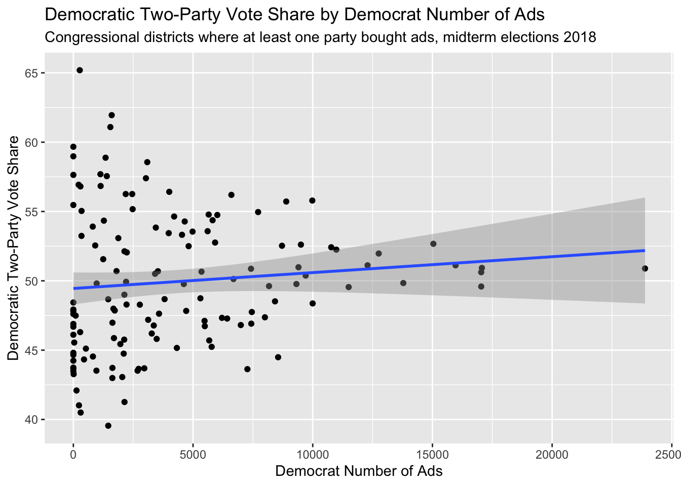
In order to visualize the effect of the air war on elections, I began by creating a scatterplot of Democratic ads and voteshare in 2018. This showed a direct correlation between higher vote share and fewer ads, leading to the inference that Democrats target their ads mostly in districts with close races.
In order to have a greater understanding of where Democratic ads were being broadcast, I also created a gradient map showing which districts have the most ads run in them.
Maps
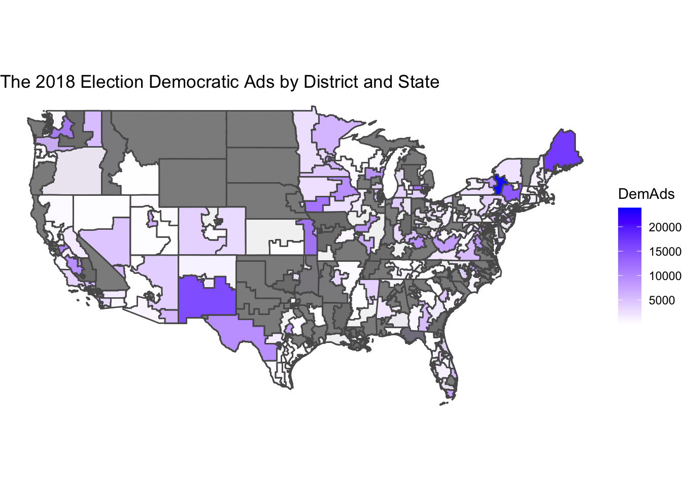 This map shows pretty clearly the accuracy of the prior scatterplot. Most Democratic ads are run in a fraction of all districts, and are highly targeted. This led me to start strategically thinking about my models. I wanted to incorporate ads while taking into account how targeted they are towards swing districts, so I coded a binary variable to indicate whether there were ads or not. I also coded a binary variable for whether there were expert ratings or not because this is another indicator of a swing district.
Conclusion
This week’s extension assignment was to fit a model and create a prediction based solely on 2018 data, then evaluate the model for limitations. The first limitation was immediately obvious to me. Whenever I filtered my “training” data to just 2018 for the model, it caused my model to give NA values despite having the values. While wonky, this makes complete sense. When we train a model, we usually use multiple years and levels of data so the model can understand patterns from which to generate a prediction.
When using just 2018 data didn’t work, I tried to make a model based on all the historical ads data that we had, plus my binary variables, but this model yielded r-squareds that were so low that they required the use of e plus some zeroes to accurately depict the small size. I tried taking out the binary variables but the r-squareds were still abysmally low. All of the data was so insignificant that R refused to use it as a basis for predictions and errored out.
I believe that this is all representative of both Gerber et al. and Huber and Arceneaux’s observations that ads have little to no effect, and I will avoid using them in the future in my observations.