Introduction

This week in Election Analytics, we will be incorporating incumbency and expert predictions into our existing models.

Incumbency is widely considered to have an impact in elections. In recent years, analysts have looked deeper into this, identifying two types of incumbent impact: President’s Party and district-level incumbency. On a district level, many have speculated that voters may reward or punish incumbency for various reasons. Adam Brown asserts, however, that voters actually do not care about the incumbent candidate. Rather, incumbency inherently enables structural advantages that favor the incumbent. For example, the incumbent has the ability to reward their district with “pork,” or economic benefits.

The President’s party tends to lose seats during congressional midterm elections, because this election is generally seen as a referendum on the president. Folke and Snyder explored this phenomenon through the lens of gubernatorial elections, ultimately finding that the party of the governor does experience losses. Folke and Snyder attributed some of these results to poor economic performance and other factors. They also ruled out reversion to the mean as the cause of the loss, indicating that it should also not be considered as much on a national level.

Turning to my work this week: First, I attempted to evaluate the accuracy of expert predictions. Expert predictions are generated by well-known election predictors and polling houses in order to provide data for their own prediction models. They are effectively refined polling data but they also take into account the fundamentals such as GDP, incumbency, and district-specific information.

Expert Predictions

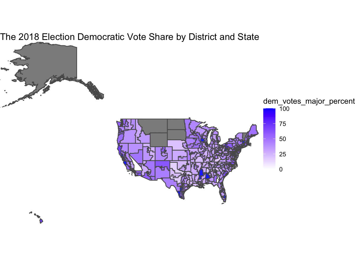
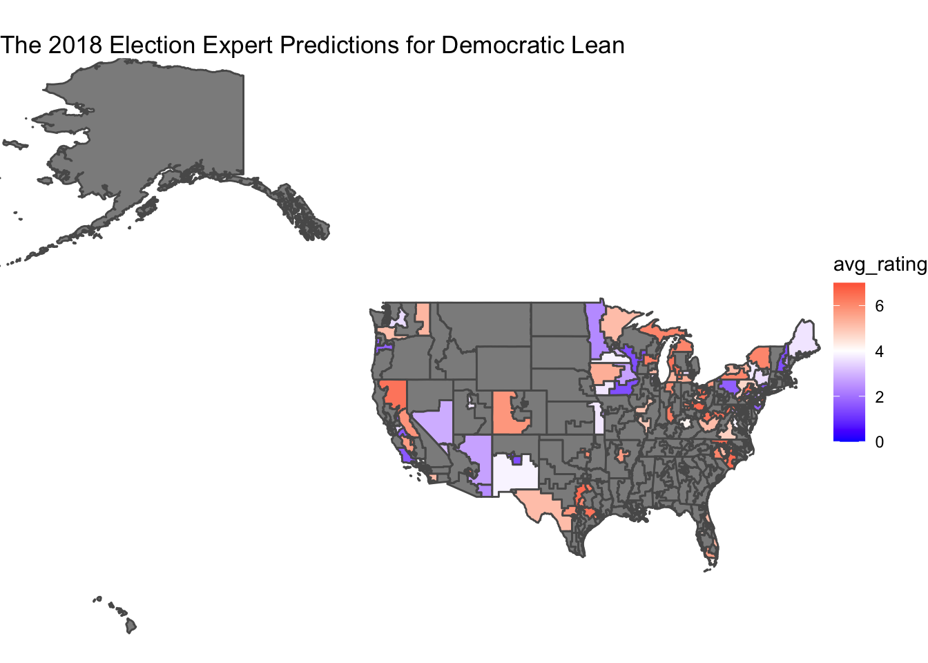
In order to compare the accuracy of the predictions, I created two maps, one of 2018 Democratic voteshare and one of the average expert ratings, where 7 is Solid R and 1 is Solid D. The issue with this is immediately obvious. We are missing so much data that the expert predictions are almost useless as a basis for anything except swing districts. From the little data we have, the average expert ratings seem to align with voteshare. Districts with lower Democratic voteshares are more likely to be shaded closer to a tossup or lean Republican. However, in a prediction, this data would only be useful in tandem with polls on the districts that don’t have expert predictions, and data on safety districts.

# Modelling

For my predictive model, I initially planned to regress on polls, economic data, expert predictions and incumbency. However, I wished to avoid accidentally overfitting my model so I cut out the economic data, considering that expert predictions often take it into account already.

I planned to join polling data with the expert prediction data in order to enhance my model like I evaluated above, however I ran into many issues with missing data so I decided that it would be more productive to predict solely the swing districts established by the expert predictions.

## Rows: 3144 Columns: 45

## ── Column specification ────────────────────────────────────────────────────────
## Delimiter: ","
## chr (28): pollster, sponsors, display_name, pollster_rating_name, fte_grade,...
## dbl (12): poll_id, pollster_id, sponsor_ids, pollster_rating_id, sponsor_can...
## lgl  (5): subpopulation, tracking, internal, nationwide_batch, ranked_choice...

## 
## ℹ Use `spec()` to retrieve the full column specification for this data.
## ℹ Specify the column types or set `show_col_types = FALSE` to quiet this message.

Finally, I also wanted to use incumbency in the regression but I ran into issues with the scope of the data set and lack of incumbency data for 2022 so for now, I’m relying on the incumbency that has already been worked into the expert predictions and in future posts, I will make it stand out a bit more in accordance with Adam Brown.

## Warning in predict.lm(object = .x, newdata = as.data.frame(.y)): prediction from
## a rank-deficient fit may be misleading

## # A tibble: 94 × 3
##    state      district  pred
##    <chr>      <chr>    <dbl>
##  1 Alaska     AL        48.0
##  2 Arizona    1         51.3
##  3 Arizona    2         49.1
##  4 Arizona    6         48.2
##  5 California 21        48.3
##  6 California 22        60.1
##  7 California 25        58.3
##  8 California 26        54.8
##  9 California 3         49.0
## 10 California 45        51.9
## # … with 84 more rows

Conclusion

Frankly, this week was a lot of trial and error. The predictions for the swing states are not horrible. The R-Squareds range from perfect 1 (probably in uncontested races) to .03 but the vast majority are in the .7-.9 range. I would rely on these given dire circumstances.