Introduction

This week in Election Analytics, the subject of discussion is Polling. How do polls impact election predictions? Are they reliable? How should they be weighed when compared to other factors like the fundamentals, or economy-based predictions? Before diving into my model and this week’s adjustments, let’s break down the work of some more experienced pollsters.

Nate Silver became almost a household name in 2008 after he successfully predicted the outcome of the presidential election in 49 out of 50 states. His blog, FiveThirtyEight, has since become a leading election prediction model, taking into consideration a wide variety of factors. FiveThirtyEight takes the attitude that if it isn’t broken, don’t fix it. They have been slightly altering the same model for years, rather than creating a new model each year. They also use nearly identical models for their House, Senate, and gubernatorial races, predicating the results for all of them on localized data rather than the statewide and national data used for presidential elections. In 1907, Francis Galton proved the wisdom of the crowds, where the mean among a large group of guesses is likely to be close to the correct answer. Silver takes this to heart and relies less on polling when the quantity of polling is few or the quality of the polling is less reliable. Silver also makes many post-game adjustments to his models, accounting for likely voters, statistical bias, and timeline. Finally, a recent comment from FiveThirtyEight notes that their recent testing has shown that partisanship and generic ballot should have more influence than other fundamentals like incumbency.

G. Elliott Morris is a data journalist for the Economist. He also manages the Economist’s election prediction model. Much like FiveThirtyEight, the Economist’s model takes into consideration polls, partisan lean, incumbency, the economy, and fundraising. Compared to Silver, however, Morris does not seem to apply the same frequent adjustments to his model (or at least does not describe them in his explanation). Morris is very aware of the tendency to over-fit models and consciously avoids this, through both cross-validation and, it seems, fewer manual adjustments. Morris also weighs polls differently than Silver. While Silver seems to calibrate polls against each other if one is consistently above or below the others, the Economist lends less weight overall to pollsters that tend to over or underestimate.

While both of these approaches are valid and lead to accurate results, I tend to favor Morris. While I prefer FiveThirtyEight’s attention to partisanship and their method of calibrating polls against each other, they seem to engage in too much manual adjustment and overfitting that seems unnecessary or misleading. I will be taking these ideas into consideration as I assemble my own model.

Modeling

Last week, I found that economic factors are a solid base for a prediction, though not a good sole factor to rely on. I decided that this was enough to warrant including economic factors in my model this week. However, I chose to use GDP over RDI because my model responded better to it during testing. In order to create this week’s model, I modified, selected, grouped, summarised, and spread datasets containing generic poll results, economic factors, and popular vote margins for 1950 through 2020. Based on Gelman and King’s article describing how polls conducted further in advance of the election are often more accurate, I also filtered the polling data to focus on polls conducted more than 90 days before election day. Finally, I was able to create a data frame for modeling and graphing. I regressed Incumbent Party Vote Share on a combination of Incumbent Average Support in generic polls and GDP growth percent. I calculated regressions for all the data together and I split it up between cases where the incumbent party won and lost.

Below, you will find two graphs, one showing the different regressions for incumbent win versus challenger win, and the other showing the regression line for all of the data together. The second graph marks in green the challenger wins.

In the first graph, neither incumbent wins nor challenger wins seem to be particularly well-correlated. In the second, the correlation seems weak but still stronger than the split set. The stargazer results back this up. The adjusted r-squared value of the incumbent-win-only regression is abysmal at 0.04815, indicating basically no correlation. The challenger-win-only regression is much stronger at 0.2001, though this would typically not be considered a strong correlation to rely on for predictions. The regression for all of the data together proved to have a stronger correlation than either of the subsets, with an adjusted r-squared value of 0.3236. This regression also had an extremely low p-value.

## ── Attaching packages ─────────────────────────────────────── tidyverse 1.3.1 ──

## ✓ ggplot2 3.3.5     ✓ purrr   0.3.4
## ✓ tibble  3.1.6     ✓ dplyr   1.0.7
## ✓ tidyr   1.1.4     ✓ stringr 1.4.0
## ✓ readr   2.1.1     ✓ forcats 0.5.1

## ── Conflicts ────────────────────────────────────────── tidyverse_conflicts() ──
## x dplyr::filter() masks stats::filter()
## x dplyr::lag()    masks stats::lag()

## 
## Please cite as:

##  Hlavac, Marek (2022). stargazer: Well-Formatted Regression and Summary Statistics Tables.

##  R package version 5.2.3. https://CRAN.R-project.org/package=stargazer

## New names:
## * `` -> ...1

## Rows: 37 Columns: 21

## ── Column specification ────────────────────────────────────────────────────────
## Delimiter: ","
## chr  (4): AreaAll, winner_party, president_party, H_incumbent_party
## dbl (16): ...1, year, R_seats, D_seats, Other_seats, total_votes, R_votes, D...
## lgl  (1): H_incumbent_party_winner

## 
## ℹ Use `spec()` to retrieve the full column specification for this data.
## ℹ Specify the column types or set `show_col_types = FALSE` to quiet this message.

## New names:
## * `` -> ...1
## * ...1 -> ...2

## Rows: 302 Columns: 10

## ── Column specification ────────────────────────────────────────────────────────
## Delimiter: ","
## chr (2): date, year_qt
## dbl (8): ...1, ...2, GDPC1, quarter_yr, quarter_cycle, year, GDP_growth_qt, ...

## 
## ℹ Use `spec()` to retrieve the full column specification for this data.
## ℹ Specify the column types or set `show_col_types = FALSE` to quiet this message.

## Rows: 4219 Columns: 13

## ── Column specification ────────────────────────────────────────────────────────
## Delimiter: ","
## chr (4): pollster, type, poll_date, party
## dbl (9): Count, sample_size, bmonth, bday, year, emonth, eday, days_until_el...

## 
## ℹ Use `spec()` to retrieve the full column specification for this data.
## ℹ Specify the column types or set `show_col_types = FALSE` to quiet this message.

## `summarise()` has grouped output by 'year'. You can override using the `.groups` argument.

## Joining, by = "year"
## Joining, by = "year"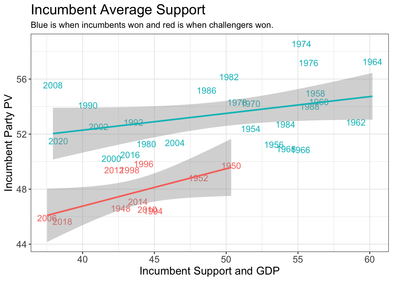

Despite its p-value, the regression on all of the data had relatively high residuals, sending mixed messages about the quality of the correlation. The regression on incumbent wins alone was not much better, but the regression on incumbent popular vote with a challenger win had a relatively low residual of about 1. This is important for our purposes because the most pressing question about the upcoming election is whether the Democrats will maintain their majority in Congress. If we can accurately predict the incumbent percent vote with a challenger win, we may be able to predict whether the Democrats will be unseated.

## Rows: 1035 Columns: 20

## ── Column specification ────────────────────────────────────────────────────────
## Delimiter: ","
## chr (10): subgroup, startdate, enddate, pollster, grade, population, multive...
## dbl  (9): samplesize, weight, influence, dem, rep, adjusted_dem, adjusted_re...
## lgl  (1): tracking

## 
## ℹ Use `spec()` to retrieve the full column specification for this data.
## ℹ Specify the column types or set `show_col_types = FALSE` to quiet this message.

## Joining, by = c("pollster", "sample_size", "dem", "rep", "year")

## Joining, by = "year"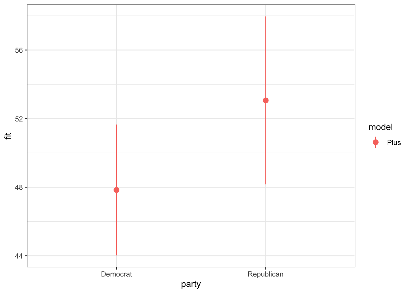

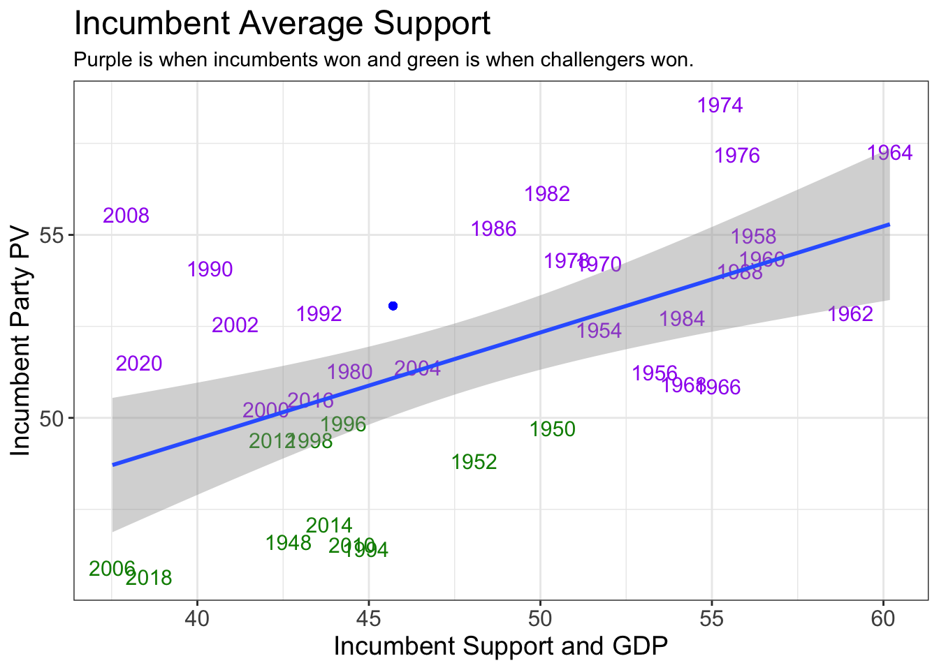Looking at the blue dot on the graph above, The final prediction based on this data is that the Democrats will win the popular vote at 53.06198, holding onto their majority. However, the upper and lower bounds on the graph of the model predictions do intersect, meaning that this prediction cannot be certain.